Conditional Formatting Excel
We’ve all been there—staring at spreadsheets filled with endless rows and columns of data, making it challenging to derive any meaningful insights. Imagine how convenient it would be if, with just a few simple tweaks, you could suddenly gain clarity and organization within these sprawling sheets. Excel Conditional Formatting offers an array of options to do just that. Often referred to as “conditional formatting” within the software, is a powerful tool for enhancing data based on specific conditions. If you’re looking to gain better insights using Conditional Formatting in Excel but aren’t sure where to start? Keep reading!
How to Use Excel Conditional Formatting?
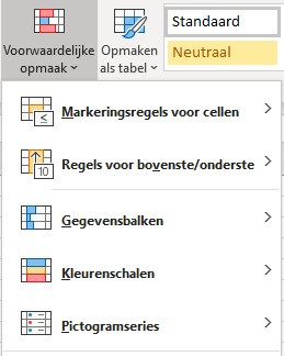
To highlight critical data points in large spreadsheets, you can utilize Excel’s Conditional Formatting feature. To set a formatting rule for a data range, first, select the data. Then, navigate to ‘Conditional Formatting’ from the start menu.
Applying New Formatting Rules in Excel
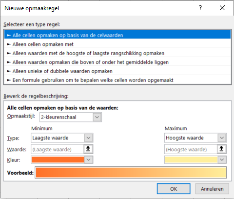
When you click on ‘New Rule,’ a menu opens, offering a wide range of formatting options. From this menu, you can choose different formatting styles depending on the data value. For instance, numbers above or below a specific value can be colored differently. You can also format cells based on their being below the average value in the data set. Even textual data can have conditional formatting applied. For example, all cells containing the word ‘yes’ can be colored green.
Additional Options for Conditional Formatting in Excel
Beyond the ‘New Rule’ option, there are five other handy choices. Each with its own set of specialized sub-options. You can format cells based on whether they are above or below a given value. Suppose you have sales figures for all your clients and want to quickly identify those exceeding a specific revenue target; this feature becomes incredibly useful. If you wish to highlight your top 10 clients, the ‘Top/Bottom Rules’ option comes in handy. You can also apply color scales to the sales figures for your clients. Choosing a darker green scale for higher sales and a darker red for lower sales. Moreover, icons can be used to spotlight particular data points.
Example of Excel Conditional Formatting
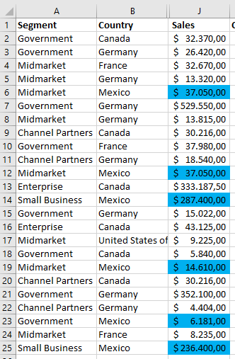
To give you a clearer understanding, let’s consider an example. If we have sales data from various countries and want to isolate sales made in Mexico, here’s how we can go about it:
Outsource Excel Tasks?
The potential of software like Microsoft Excel is immense. With efficient use, much time and effort can be saved. However, expertise is required to tap into this potential fully. Fortunately, we have that expertise at Bouwmeester Consultancy. We are more than capable of assisting you in this area. Feel free to contact us for a no-obligation discussion about the various options available. We’re eager to assist you and take the burden off your hands for all your Excel-related questions and challenges.


